
Digital Soil Mapping (DSM)
The use of geospatial techniques for mapping soils is broadly covered by the term “digital soil mapping” (DSM).
Definitions of Digital Soil Mapping
“The creation and the population of a geographically referenced soil database generated at a given resolution by using field and laboratory observation methods coupled with environmental data through quantitative relationships.” - The International Working Group on Digital Soil Mapping (WG-DSM)
“Production of soil class or property maps using GIS and/or Remote Sensing software” – anonymous
Digital soil mapping (DSM) represents “the creation and population of spatial soil information systems by the use of field and laboratory observational methods coupled with spatial and non-spatial soil inference systems” (Digital Soil Mapping: An Introductory Perspective 2007. Edited by P. Lagacherie, A. B. McBratney & M. Voltz, 2007 Elsevier 600 pages ISBN 0-444-52958-6). Soil science, geographic information science, quantitative methods (statistics and geostatistics) and cartography are combined within the DSM framework. DSM methods are used to estimate the spatial distribution of soil classes (e.g., soil series) and/or soil properties (e.g., soil organic matter), and can be employed at various scales (from individual fields to countries), and have proven valuable for developing more quantitative, more accurate, and more precise soil maps.
What is Digital Soil Mapping and How Does It Compare to Conventional Soil Mapping?
[Based on excerpts from the Digital Soil Mapping chapter in the Soil Survey Manual (2017) and “Options for Communicating Soil Knowledge” (NCSS Newsletter Issue 78, Feb 2017)]
The use of geospatial techniques for mapping soils is broadly covered by the term “digital soil mapping” (DSM). Digital soil mapping is defined as the creation of geographically referenced soil databases based on quantitative relationships between spatially explicit environmental data and measurements made in the field and laboratory (McBratney et al., 2003). Use of digital soil mapping techniques has progressed as soil scientists have adopted the latest tools to assist in the mapping process. The process of making an inference about a landscape segment (e.g., a soil map unit) from a few point-based observations using the operative soil-forming factors is “modeling.” Whether the soil map is produced using nothing but a bucket auger and an aerial photo or using geospatial software, the process is a modeling operation. The use of DSM methods is increasing over time and will eventually cease to be considered distinct, novel techniques.
The digital soil map is a raster-based map composed of 2-dimensional cells (pixels) organized into a grid in which each pixel has a specific geographic location and contains soil data. Digital soil maps illustrate the spatial distribution of soil classes or properties and can document the uncertainty of the soil prediction. Digital soil mapping better captures observed spatial variability and reduces the need to aggregate soil types based on a set mapping scale (Zhu et al., 2001). Digital soil mapping can be used to create initial soil survey maps, to complete MLRA update projects, and generate soil interpretations. It can facilitate the rapid inventory, re-inventory, and project-based management of lands in a changing environment.
The availability and accessibility of geographic information systems (GIS), global positioning systems (GPS), remotely sensed spectral data, topographic data derived from digital elevation models (DEMs), predictive or inference models, and software for data analysis have greatly advanced the science and art of soil survey. Conventional soil mapping now incorporates point observations in the field that are geo-referenced with GPS and digital elevation models visualized in a GIS. However, the important distinction between digital soil mapping and conventional soil mapping is that digital soil mapping utilizes quantitative inference models to generate predictions of soil classes or soil properties in a geographic database (raster). Models based on data mining, statistical analysis, and machine learning organize vast amounts of geospatial data into meaningful clusters for recognizing spatial patterns.
A significant amount of the data used in digital soil mapping can be archived in a digital format in a GIS, so the expert knowledge used to predict soil distribution on the landscape is retained. Objective sampling plans can be implemented to statistically capture variability of the landscape, represented by digital environmental covariates (environmental data representing soil forming factors). The most exciting aspects of digital soil mapping relate to the ability of depicting smaller segments of the landscape for traditional soil classes, continuous representation of physical and chemical properties in multiple dimensions and the associated generation of raster layers representing respective uncertainties. These are capabilities that will allow soil scientists to more completely and thoroughly represent their soil knowledge to users than the current vector model.
Digital Soil Mapping in a Nutshell
- Digital soil mapping is the generation of geographically referenced soil databases based on quantitative relationships between spatially explicit environmental data and measurements made in the field and laboratory (McBratney et al., 2003).
- Digital soil mapping is the prediction of soil classes or properties from point data using a statistical algorithm.
- The digital soil map is a raster composed of 2-dimensional cells (pixels) organized into a grid in which each pixel has a specific geographic location and contains soil data.
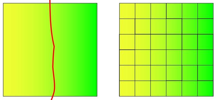
- In conventional mapping, the primary question is “Where is the boundary between two soils?” and the focus is on those marginal areas (left figure below).
- In digital soil mapping, the central concept is well defined with variation expressed across the landscape (right figure below).
- Digital soil maps illustrate the spatial distribution of soil classes or properties and can document the uncertainty of the soil prediction.
- Digital soil mapping can be used to create initial soil survey maps, refine or update existing soil surveys, generate specific soil interpretations, and assess risk (Carré et al., 2007).
- It can facilitate the rapid inventory, re-inventory, and project-based management of lands in a changing environment.
NCSS Digital Soil Mapping
The National Soil Survey Center – Geospatial Research Unit has identified DSM as an important area of focus in support of soil survey activities. Numerous DSM research projects have been supported by the GRU. Numerical classification (hierarchical and fuzzy), spatial and temporal interpolation (geostatistics, wavelets), sampling design (model vs. design based), statistical analysis (visualization, ordination, regression, and classification), uncertainty analysis (error propagation, accuracy assessment), and incorporation of auxiliary data (proximal and remotely sensed imagery, soil-terrain modeling) are among the methods used to develop predictive maps of soil classes and soil properties.
DSM Influenced Vector Soil Mapping (SSURGO)
Florida
- FL615 MLRA 156A - Water Conservation Area, Florida
Minnesota
- MN031 Cook County, Minnesota
- MN075 Lake County, Minnesota
- MN115 Pine County, Minnesota
- MN613 St. Louis County, Minnesota, Crane Lake Part
- MLRA 102A - Fergus Falls Till Plain Formdale Catena Study, Re-correlation and Investigations
- MLRA 88 - Glacial Lake Plain Baudette Catena
- MLRA 90A - Mille Lacs Uplands Coarse-Loamy Basal Till Investigation
- MLRA 88 - Glacial Lake Plain Zimmerman and Wawina Dune Influenced Catenas
North Dakota
- MLRA 55A - Barnes series - Investigation of Souris Lobe, Soil-Water Monitoring, and Map Unit Recorrelation
- MLRA 55A - Investigation of the Leeds Lobe and Map Unit Recorrelation
Texas
- TX377 Presidio County, Texas
- TX625 Guadalupe Mountains National Park, Texas
- TX626 Culberson County, Main Part, Texas
- TX627 Hudspeth County, Main Part, Texas
Utah
- UT601 Box Elder County, Utah, Western Part
- UT602 Box Elder County, Utah, Eastern Part
- UT607 Davis-Weber Area, Utah
- UT611 Tooele Area, Utah – Tooele County and Parts of Box Elder, Davis and Juab Counties
- UT612 Salt Lake Area, Utah
- UT617 West Millard-Juab Area, Utah, Parts of Millard and Juab Counties
- UT623 Emery Area, Utah, Parts of Emery, Carbon, Grand, and Sevier Counties
- UT625 Emery Area, Utah, Parts of Emery, Carbon, Grand, and Sevier Counties
- UT626 Beaver County, Utah – Western Part
- UT628 Sevier County Area, Utah
- UT629 Loa-Marysvale Area, Utah, Parts of Piute, Wayne, and Garfield Counties
- UT686 Grand Staircase-Escalante National Monument Area, Parts of Kane and Garfield Counties, Utah
Vermont
- VT009 Essex County, Vermont
Washington
- WA774 North Cascades National Park Complex, Washington
Wyoming
- WY719 Johnson County, Wyoming, Northern Part
DSM Raster Soil Survey (RSS) Projects
Minnesota
- Boundary Waters Canoe Area Wilderness (BWCA_10-DUL17)
- MLRA 102A - Fergus Falls Till Plain Formdale Catena Study, Re-correlation and Investigations (FFTP_10-FAR19)
- MLRA 88 - Glacial Lake Plain Baudette Catena (BAUD_10-BEM19)
- MLRA 90A - Mille Lacs Uplands Coarse-Loamy Basal Till Investigation (MLCU_10-DUL19)
North Dakota
- MLRA 55A - Barnes series - Investigation of Souris Lobe, Soil-Water Monitoring, and Map Unit Recorrelation (SOUR_10-DVL17)
- MLRA 55A - Investigation of the Leeds Lobe and Map Unit Recorrelation (LEED_10-BIS20)
Vermont
- Essex County, Vermont
- Fact Sheet